Noise Your Prompt: Improved Conditional Generation in Diffusion Language Models
We offer a simple modification to training continuous diffusion language models that leads to improvements in both accuracy and generation diversity on combinatorial reasoning benchmarks.
Updates:
- Our paper with full details now accepted to the COLM 2026 NonAR workshop can be read here.
- The code to reproduce the experiments are here.
- Check out our interactive demo demonstrating our method on Sudoku solving here.
Diffusion language models generate text by starting from a sequence of complete noise and then iteratively denoising the sequence over time to get a text sequence. However, most of language modelling in practice is conditional generation where the user supplies a conditioning prompt and expects a generated response based on that prompt.
Default: Keep the prompt clean
The accepted practice for conditional generation in continuous diffusion and flow language models is to simply paste in the conditioning prompt tokens during sampling: at every sampling step, make sure to replace the tokens in the sequence with the supplied prompt.
Likewise, during training, the standard practice is to paste in the conditioning prompt tokens for the noised input sequences, so the model trains with all the information from the conditional prompt (in additional to the remaining noised sequence).
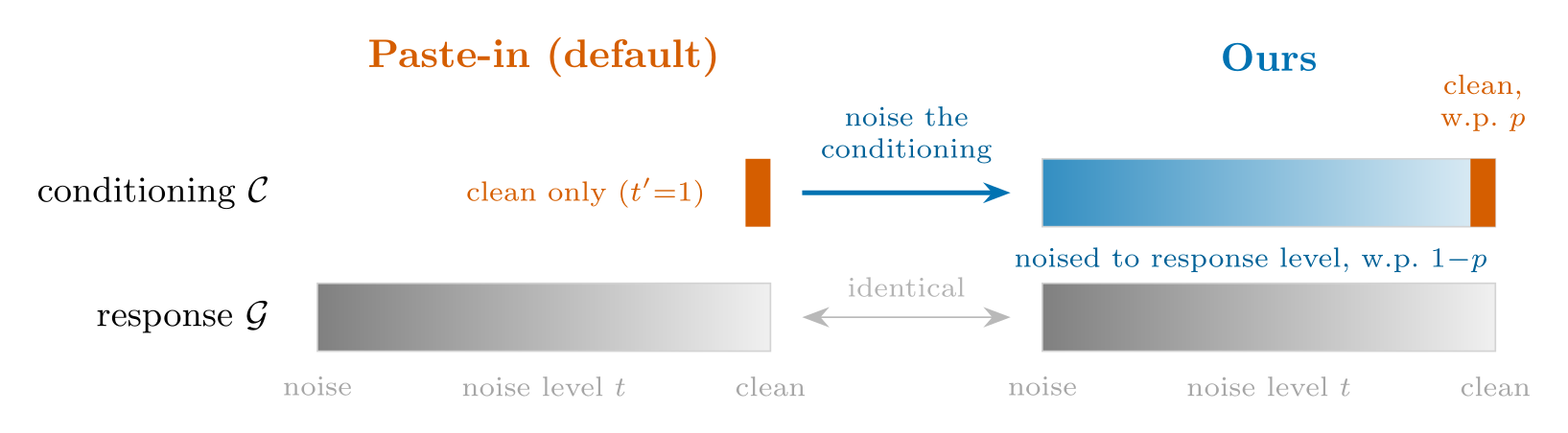 Figure 1. Our training objective. Standard "paste-in" training (left) keeps the conditioning prompt clean (\(t = 1\)) throughout corruption. We instead noise the prompt to the same level as the response with probability \(1 - p\) (right). At sampling time, both methods hold the prompt clean.
Our modification: also noise the prompt
We investigate this accepted practice of not noised the prompt. Our modification is simple: during training, also noise the prompt.
Our intuition stems from seeing what the diffusion denoising objective is doing: the model needs to predict a clean denoised version of various degrees of noised input.
More precisely, we train across different sampled times \(t \sim U[0,1]\) which define the noise corruption level of the input.
When we sample little noise \(t \to 1\), our denoising prediction problem \(f(x_t) \to x_1\) is easy: our input is basically already the denoised solution. When we sample a lot of noise \(t \to 0\), our prediction problem is very difficult: we have little signal to predict the denoised version from.
So by training with a variety of noise levels, our model is exposed to a variety of task difficulties.
But for conditional generation, we are supplied with a prompt \(x\) and we need to generate a corresponding response \(y\). And the standard practice is to never noise the prompt \(x\), so the model uses a fully clean prompt to make a prediction.
But we see this as sub-optimal: in cases where the response \(y\) is heavily determined by the prompt \(x\), the model can be over-reliant on the input prompt; by additionally noising \(x\) we can train the model on various degrees of conditional prediction tasks (increasing the noise on the prompts increases the task difficulty); and if we noise the prompt \(x\) we can also include the model's denoised prediction of the prompt in the loss.
The method, explained trivially
The method is simple to implement. With a probability \(p < 1\), we also noise the conditioning prompt tokens along with the rest of the sequence. Else, we keep the prompt tokens clean (we paste the clean prompt in).
Results
On Sudoku, lower p gives higher solve rates. Training with noised prompts is even more effective on more difficult puzzles (difficulty hard). We also visualize the solution progression (by reading off its denoised \(x_1\) predictions) over the sampling steps: noised prompt training allows the model to saturate and reach its max solve rate faster.
Table 1. Sudoku solve rate (%) on 2,000 held-out puzzles, trained on 10,000 puzzles. Lower \(p\) (noising the prompt more often) gives higher accuracy on both difficulties.
| Training setting | Easy (40/81 clues) | Hard (30/81 clues) |
|---|---|---|
| paste-in (p = 1.0) | 68.5 | 3.7 |
| noised (p = 0.5) | 87.5 | 14.7 |
| noised (p = 0.2) | 88.9 | 24.3 |
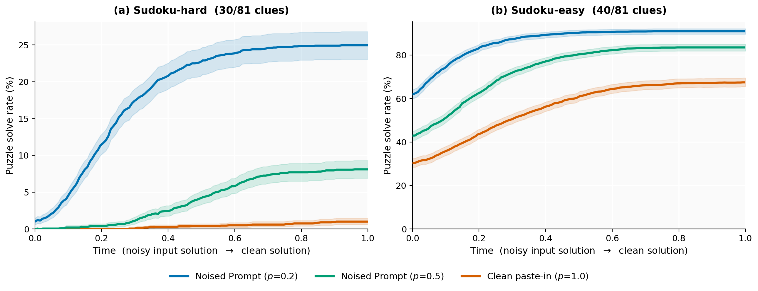
Figure 2. Puzzle solve rate along the sampling trajectory (noisy input → clean solution), read from the model's \(x_1\) prediction at each step over 2,000 held-out puzzles. The noised-prompt models (\(p = 0.2, 0.5\)) reach a higher solve rate and saturate earlier than paste-in (\(p = 1.0\)).
Interactive. Ten hard puzzles drawn at random from a held-out set of 128, solving in parallel under both methods from the same seeded noise; a board's border turns green the moment it is fully solved. The noised-prompt model (\(p = 0.2\)) solves more, and earlier, than paste-in (\(p = 1.0\)). Hit resample for a fresh draw, or open it full screen.
In N-Queens, there are multiple possible valid solutions for a given input board. This allows us to track the model's generation diversity: how much of the possible valid solutions does it generate.
Table 2. N-Queens accuracy and coverage (%) over 750 held-out boards with 20 generations each. Noising the prompt improves both metrics, with the largest coverage gains on the harder \(10\times10\) boards.
| Training setting | Acc. (8×8) | Coverage (8×8) | Acc. (10×10) | Coverage (10×10) |
|---|---|---|---|---|
| paste-in (p = 1.0) | 97.7 | 88.1 | 84.8 | 49.9 |
| p = 0.5 | 99.0 | 90.9 | 94.2 | 60.7 |
| noised (p = 0.2) | 99.2 | 93.0 | 97.9 | 73.9 |
Training with noised-prompts significantly increases coverage of possible valid solutions, while also increasing solution accuracy.
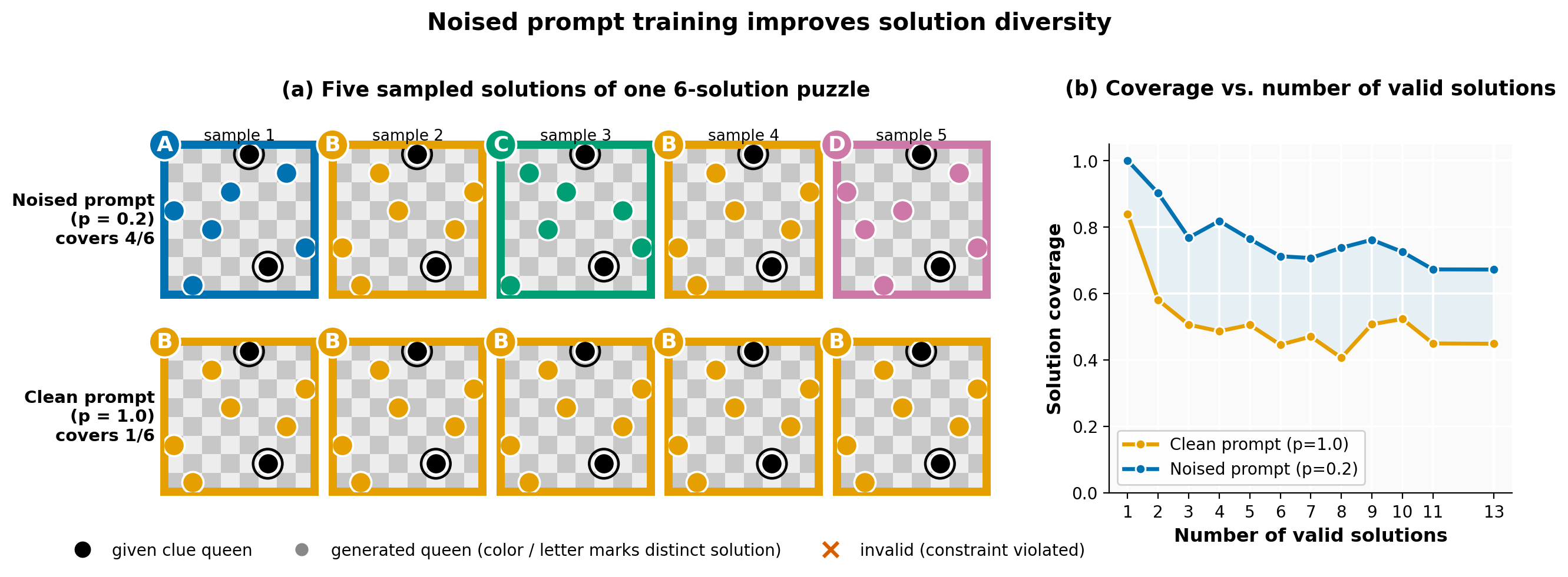
Figure 3. Noising the prompt improves solution diversity. (a) Generations for one held-out \(8\times8\) board with six valid solutions: the noised-prompt model (\(p = 0.2\)) spreads across the solution set, while paste-in (\(p = 1.0\)) collapses onto a single completion. (b) Coverage vs. the number of valid solutions admitted by the board, over 750 held-out \(10\times10\) puzzles; the noised-prompt model dominates at every solution count.
While a low probability of seeing clean prompts works well, some probability is necessary. Training only noised prompt tokens (fully unconditional training) fails as it does not know how to use the clean prompt tokens during inference.
Table 3. Fully unconditional training (\(p = 0.0\)) fails — with the prompt always noised, the model never learns to use the clean prompt supplied at inference.
| Fully unconditional training (p = 0.0) | Accuracy |
|---|---|
| Sudoku easy | 1.5 |
| Sudoku hard | 0.0 |
Relation to Classifier Free Guidance
Classifier-free guidance trains with a binary inclusion/exclusion of the conditioning information.
Our method can be seen as a continuous generalization, where the amount of conditioning information is a spectrum (full noise \(t=0\) mimics exclusion, zero noise \(t=1\) mimics inclusion, intermediate noise \(t\) is a mixture).
However, in this work, we only noise the conditioning prompt during training: during sampling, we keep the conditioning prompt tokens clean. Combining predictions under fully clean conditioning tokens and partially noised conditioning tokens during sampling may be a natural next direction.
Conclusion
Continuous diffusion language models are exciting models with nice properties: unlike AR models, they are easily controllable. Recent work has boosted their unconditional generation quality. Here we show that making a simple modification to training (also noise the prompt), we see improvements to accuracy and diversity of generation on combinatorial reasoning benchmarks like Sudoku and N-Queens.
At Lateral Intelligence, we are working towards advancing the next generation of language modelling with more natively controllable language models. We're a small team based in San Francisco.
If you're building in this direction and want to join, reach out at join@lateralintelligence.org.
If you're interested in supporting the work, get in touch at invest@lateralintelligence.org.